Professor Baragar studied the automorphism group of a Wehler $K3$ surface with Picard number three in his 2003 article Orbits of curves on certain K3 surfaces.
The surface $X$ studied by Baragar has a Néron-Severi group $\text{NS}(X)$ with Gram matrix $$Q_{\mathcal{D}} = \begin{bmatrix} 2 &4 & 1 \\ 4 &2 & 0 \\ 1 & 0 & -2 \end{bmatrix}$$with respect to a fixed basis $\mathcal{D}$.
It should be noted that Baragar applies two successive changes of bases $$\mathcal{D} \longrightarrow \mathcal{D}^\ast \longrightarrow \mathcal{B}^\ast$$ under which elements $M\in O(\NS(X)$) initially expressed with respect to $\mathcal{D}$ are turned into transformations with respect to a basis $\mathcal{B}^\ast$ by $$M \longmapsto (SQ_{\mathcal{D}})M(Q_{\mathcal{D}}^{-1}S^{-1})$$with $$S = \begin{bmatrix} 1 & 0 & -1 \\ 0 &1 & -1 \\ 0 & 0 & 1 \end{bmatrix}.$$
Thus considering matrices with respect to the basis $\mathcal{B}^\ast$, Prof Baragar states that $$T_1 = \begin{bmatrix} 0 & 0 & 1 \\ 3 &-1 & 3 \\ 1 & 0 & 0 \end{bmatrix}, \qquad T_2 = \begin{bmatrix} -1 & 4 &1 \\ 0 & 1 & 0 \\ 0 & 0 & 1 \end{bmatrix}$$ are elements of $\aut(X)$ and also indicates that the matrix $$T_3 = \begin{bmatrix} 5 & 14 & -20 \\ 4 & 15 & -20 \\ 4 & 14 & -19 \end{bmatrix}$$ could also be an automorphism but that this fact cannot be asserted with certainty.
We now show that applying our computer-based algorithmic approach to this $K3$ surface will provide an answer to Prof. Baragar’s interrogation regarding the matrix $T_3$ and enable us to obtain a lot of factual information regarding this surface.
We will start by using the Poolized Borcherds’ method to compute a generating set of $\aut(X)$ and show that each of the transformations $T_1$, $T_2$ are indeed elements of $\text{Aut}(X)$. We will then deal with $T_3$. Note that we will also put to use some of the other solutions produced during this thesis to do a further study regarding Baragar’s Picard $3$ Wehler $K3$ surface: Computation of a Hilbert basis of a fundamental domain of the action of $\aut(X)$ onto $\nps$, i.e., the Hilbert basis of a chunk of the Nef cone, graphical representation of this fundamental domain…
Before proceeding further, let’s write $T_1$, $T_2$ and $T_3$ with respect to the basis $\mathcal{D}$ for $\NSX$ under which a Gram matrix for this lattice is the matrix $$Q_{\mathcal{D}} = \begin{bmatrix} 2 &4 & 1 \\ 4 &2 & 0 \\ 1 & 0 & -2 \end{bmatrix}$$ provided by Baragar in his article.
Starting from a matrix transformation expressed with respect to the basis $\mathcal{B}^{\ast}$, the transformation $$ M \longrightarrow Q_{\mathcal{D}}^{-1} S^{-1} M S Q_{\mathcal{D}}$$ turns $M$ into matrix transformation expressed with respect to the basis $\mathcal{D}$.
First and foremost, let’s deal with conventions : We have to take into account the fact that Prof. Baragar uses the convention that elements of $M\in O(\NSX)$ expressed with respect to $\DD$ satisfy $$M^t Q_{\mathcal{D}} M = Q_{\mathcal{D}} $$ while we adopted the convention that transformations $M\in O(\NSX)$ transformations satisfy $$ M Q_{\mathcal{D}} M^t = Q_{\mathcal{D}}.$$ We will thus take the transpose of each matrix obtained after applying the above mentioned change of basis. Still keeping the notation $T_i$ for $i=1,2,3$ to denote Professors Baragar’s matrices expressed with respect to the basis $\mathcal{D}$, we apply the above mentionned change of basis from $\mathcal{B}^\ast$ to $\DD$ and take the transpose of each of the matrices thus obtained. Doing so enables us to obtain$$T_1 = \begin{bmatrix}1 & 0 & 0 \\ 4 & -1 & 0 \\ 1 & 0 & -1\end{bmatrix}, \qquad T_2 = \begin{bmatrix} -1 & 4 & -1 \\ 0 &1 & 0 \\0 & 0 &1 \end{bmatrix}$$and $$T_3 = \begin{bmatrix}5 & 14 & -20 \\ 4 & 15 & -20 \\ 4 & 14 & -19\end{bmatrix}.$$
We now go back to the familiar notations used along with our thesis and forget about the matrix $S$ introduced by Baragar, which will be of no use during the remainder of our study.
As usual, we define $S = \NS(X)$.
Computation of the automorphism group of $X$
We follow the guidelines provided in
Setting up the environment to execute the Borcherds’ method
to set up an environment that will enable us to apply the Poolized Borcherds’ method to $X$ and compute a generating set of $\text{Aut}(X)$. We will soon show that Baragar’s surface fits within the framework under which obtaining a generating set of $\aut(X)$ by applying the Borcherds’ method is guaranteed.
As indicated on the page mentioned above, we need knowledge of :
- A Gram matrix $G_S$ of $S$, which Professor Baragar here provides as $G_S = Q_{\mathcal{D}}$.
- A primitive embedding of $S$ into $\mathbb{L}=U\oplus E_8(-1)$ should not be very difficult to obtain since $X$ as Picard $3$, so only three vectors have to be determined.
- An initial ample class.
One can easily verify that the elements $$v_1 = [1,1,0,0,0,0,0,0,0,0], \; \, v_2 = [2, 2, 0, 0, 1, 2, 0, 0, 0, 0] \; \ \text{and} \,\; v_3 = [0, 1, 0, 0, 0, 0, -1, 0, 0, 0]$$ define a primitive embedding of $S$ into $\mathbb{L}$ given by $$ \iota : [x_1 , x_2, x_3] \in S \longmapsto \alpha_1 v_1 + \alpha_2 v_2 + \alpha_3 v_3 \in \mathbb{L}$$ and applying the guidelines provided in the section 2.3 of our thesis Finding an initial ample class enables us to assert that the class $[1000,-100,-1]$ can be taken as initial ample class.
If you have access to our demo server, please open a Sage console from the folder ThesisPrograms and proceed as follows to load a ready-to-use input data list for the surface under study :
INPUT_DATA=load('INPUT_DATA/DEMO/INPUT_DATA_BARAGAR_SURFACE_PICARD_3.sobj')

Instead of directly loading borcherds_direct, we will proceed step-by-step, as described in this figure.
We start by loading init_emb to automatically set up an initial environment suitable for the preliminary checks, which must be done before executing Borcherds’ method.
load('init_emb.sage')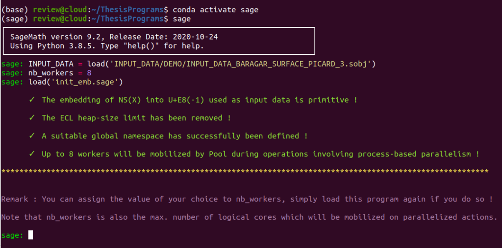
We then determine whether the Borcherds’ method will return a generating set of $\text{Aut}(X)$ by running ker_checker :
load('ker_checker.sage')
Fine. We now check whether the initial embedding of $S$ into $\mathbb{L}$ defined by the vectors $v_1,v_2$ and $v_3$ (which has automatically been defined by init_emb) enables us to get an initial nondegenerate chamber $\mathcal{D}_0$ from which the Borcherds’ method can start the exploration of the $\ps$-chamber structure over $\nps$.
To this end, we load degentest :
load('degentest.sage')
Great! Had the answer been negative, loading emb_updater would have enabled us to update our initial embedding. Note that if an application of emb_updater for which using the ample class $[1000,-100,-1]$ as input data results in a failure, we can take advantage of AmpTester to find another suitable ample class enabling us to succeed in updating our embedding.
We explain how to do so on this page or here.
All lights are green for us to launch the Borcherds’ method.
First, we define two string variables, text1 and text2, to personalize the folder name and files in which the various reports, data files, and recovery data produced by our implementation of Borcherds’ method will be stored, as discussed here.
text1 = str('baragar_picard_3')
text2 = str('demo')
The folders and files created by the method during the study of Professor Baragar’s surface will have names following the pattern some_data_baragar_picard_3_demo.
Note that randomly chosen English words will automatically be assigned to text1 and text2 if you forget to do so yourself.
We launch the Poolized Borcherds’ method :
load('borcherds.sage')
Two minutes are enough for the program to determine a generating set of $\aut(X)$ along with an upper bound on the number of orbits of smooth rational curves on $X$ under the action of $\text{Aut}(X)$.

The Poolized Borcherds’ method thus returns that the matrices $$g_1= \begin{bmatrix} 1 & 0 & 0 \\ 4 & -1 & 0 \\ 1 & 0 & -1 \end{bmatrix}, \quad g_2=\begin{bmatrix} 14 & -4 & 1 \\ 52 & -15 & 4 \\ 13 & -4 & 2 \end{bmatrix}, \quad g_3 =\begin{bmatrix} 41 & -14 & 20 \\ 120 & -41 & 60 \\ 0 & 0 & 1 \end{bmatrix}$$ form a generating set of $\aut(X)$ and that there are at most two orbits of the set of smooth rational rational curves on $X$ under the action of $\text{Aut}(X)$. Note that the method also returned the data of a fundamental domain of the action of $\aut(X)$ onto $\nps$ which consists in the union of the twenty-seven $\ps$-chambers each representing their own congruence class of chambers contained in $\nps$ under the action of $\aut(X)$.
NB: the data of these chambers is stored under the name LOSOC,
in which are stored representatives sorted by level.
Take LOSOC = sum2(LOSOC) to obtain the list of chambers.
Borcherds’ method produced a fundamental domain of a nice chunk of $\nps$ under the action of $\aut(X)$.
As mentioned at the beginning of this page, our goal is to retrieve Prof. Baragar’s results and obtain answers to the questions left in the wake of his article.
Baragar found that $$T_1 = \begin{bmatrix}1 & 0 & 0 \\ 4 & -1 & 0 \\ 1 & 0 & -1\end{bmatrix}, \qquad T_2 = \begin{bmatrix} -1 & 4 & 1 \\ 0 &1 & 0 \\0 & 0 &1 \end{bmatrix}$$ were elements of $\aut(X)$ and was not able to assert with full certainty that $$T_3 = \begin{bmatrix}5 & 14 & -20 \\ 4 & 15 & -20 \\ 4 & 14 & -19\end{bmatrix}$$ was also in $\aut(X)$.
The Borcherds’ method provides direct confirmation regarding $T_1$ : $$T_1 = g_1$$where ${g_1,g_2,g_3}$ is the generating set returned by the method.
Since we obtained a generating set of $\aut(X)$, we should be able to express $T_2$ as a word $$ g_{i_1}g_{i_2}\dots g_{i_k}$$ with for some integers $k\in \ZZ$ and $i_1,\dots,i_k\in \{1,2,3\}$ formed from the generators $g_1,g_2,g_3$ returned by the Borcherds method (which are of order $2$, i.e. equal to their own inverse) Define
T1 = Matrix([[1,0,0],[4,-1,0],[1,0,-1]]);
T2 = Matrix([[-1,4,1],[0,1,0],[0,0,1]]);
T3 = Matrix([[5,14,-20],[4,15,-20],[4,14,-19]])
so that we can work with Baragar’s matrices $T_1,T_2$ and $T_3$.
The borcherds.sage program automatically stores the set of generators obtained by the Borcherds’ method under the variable GAMMA :

Let’s take advantage of the knowledge of these generators to compute a large set of elements of $\text{Aut}(X)$ will provide some ground for our search for $T_2$ and $T_2$.
For example, we compute the set of all words of length inferior or equal to $5$, which can be formed from the elements of GAMMA.
Let
GID = GAMMA+[matrix.identity(3)]and
WORDS=[(a,b,c,d,e,a*b*c*d*e) for a in GID for b in GID for c in GID for d in GID for e in GID]Note that the elements of [q[5] for q in WORDS] are the words themselves and form a subset of the set of all elements of $\aut(X)$.
Use
WORDS = duplikiller(WORDS)in order to remove duplicates from the list WORD. We already now that $T_1 \in \aut(X)$, since it is in the generating set returned by the Borcherds’ method. Let’s test $T_2$ and $T_3$ for membership in [q[5] for q in WORDS] :
T2 in [q[5] for q in WORDS]
Great, $$T_2 \in \aut(X)$$ ! Let’s find how $T_2$ can be expressed in terms of $g_1,g_2,g_3$.
Enter
WORDS[[q[5] for q in WORDS].index(T2)]
Thus $$T_2 = g_1^3 g_2 g_1.$$ Using the fact that $g_i^2 = \id$ for $i=1,2,3$ we have $$T_2 = g_1 g_2 g_1 = g_1 g_2 g_1^{-1}$$ that is, $T_2$ is obtained by conjugation of $g_2$ by $g_1$.
Let’s check whether an answer to Baragar’s interrogation can now be provided regarding $T_3$.
Before proceeding further, note that we can first check whether $T_3$ fulfills all the conditions to be an automorphism by using the function AutTester. See section 1.6.2 of our thesis for more details.
AutTester(T3)If AutTester returns false, we will now for sure that $T_3 \notin \aut(X)$.

Fine! We know that $T_3$ fulfills the conditions required for it to be an element of $\aut(X)$.
Let’s check whether $T_3$ belongs to [q[5] for q in WORDS] :
T3 in [q[5] for q in WORDS]
GREAT ! We have the confirmation that $T_3 \in \aut(X)$ !
Let’s take a look at how $T_3$ can be obtained from the generators of $\aut(X)$ returned by the Borcherds’ method. Typing
WORDS[[q[5] for q in WORDS].index(T3)]returns

so that we thus have
$$T_3 = g_1^3 g_3 g_1 = g_1 g_3 g_1.$$
That is, $T_3$ is obtained by conjugation of $g_3$ by $g_1$.
We thus see that the solutions developed during this thesis enabled us to obtain an answer to Baragar’s twenty years old questions:
Does $T_3 \in \aut(X)$ ?
The answer is indeed positive.
But that is not all! Remember that the Borcherds’ method returned a fundamental domain of the action of $\nps$ under $\aut(X)$. Let’s use our program fundamentalizer to obtain interesting geometric information about this fundamental domain, such as a Hilbert basis or a graphical representation.
load('fundamentalizer.sage')The program fundamentalizer starts with an analysis of the walls of each chamber forming the fundamental domain to obtain a precise characterization of its geometry in $\nps$.
Indeed, fundamentalizer‘s will try to compute a Hilbert basis of this chunk of the $\text{Nef}$ cone!
Fundamentalizer readily returns that a Hilbert basis for the cone associated to the fundamental domain with an intersection matrix :

That is, the elements $$\left[6, -2, 3\right], \left[6, -1, 3\right], \left[3, -1, 1\right], \left[4, -1, 0\right], \left[5, 1, -3\right], \left[3, 0, -1\right], \left[1, 0, 0\right], \left[4, -1, 2\right]$$ of $\NS(X)$ form an Hilbert basis of the cone associated to the fundamental domain returned by the Borcherds’ method, with intersection matrix $$\begin{bmatrix} 2 & 22 & 1 & 8 & 55 & 21 & 7 & 8 \\ 22 & 44 & 11 & 22 & 77 & 33 & 11 & 22 \\ 1 & 11 & 0 & 2 & 22 & 8 & 3 & 4 \\ 8 & 22 & 2 & 2 & 22 & 8 & 4 & 10 \\ 55 & 77 & 22 & 22 & 44 & 22 & 11 & 44 \\ 21 & 33 & 8 & 8 & 22 & 10 & 5 & 18 \\ 7 & 11 & 3 & 4 & 11 & 5 & 2 & 6 \\ 8 & 22 & 4 & 10 & 44 & 18 & 6 & 10 \end{bmatrix}.$$
Having a Hilbert basis of a chunk of the NEF cone can always be helpful; one never knows!
Let’s try to obtain a graphical representation of this fundamental domain.
Set PLOT_BOOL = True and relaunch fundamentalizer
PLOT_BOOL = True
and get a nice visual representation, which, after a little bit of post-processing, renders as

We can see that there are indeed two $(-2)$-walls.
Let’s compute some data regarding classes of smooth rational curves on $X$.
Load our complete solution pack proj_mod for the study of projective models of $K3$ surfaces.
load('proj_mod.sage')First, we need to find another ample class. The current ample class amp0 in the global namespace is too “big”: Given an ample class $P_0$, integers $d$ and $m$, and a Gram matrix of $\NS(X)$, the program CGS, which is based on Professor Xavier Roulleau’s Magma program SmoothRationalCurves, will return the set
$$\{D\in \NS(X) \mid D^2 = d, \; D\cdot P_0 \leq m\}$$
and returns classes $D$ of smooth rational curves when $d=-2$ through an additional sorting based on a Vindberg algorithm, see Roulleau’s article or this article due to Lairez and Sertoz for more details.
The class amp0 that we used until now $$[1000,-100,-1]$$ will force us to set a large value for the parameter $m$ to obtain at least a few classes of smooth rational curves; we thus need a “smaller ample class”.
Let’s test the class $[10,-1,-1]$ for ampleness by using our program AmpTester :
AmpTester(Matrix([10,-1,-1])) 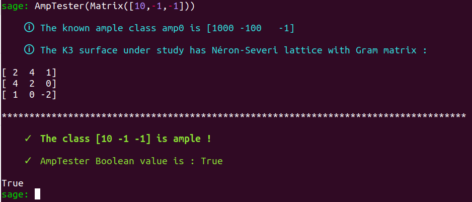
Great! Let’s replace our previous ample class with $[10,-1,-1]$ in the global namespace :
amp0 = Matrix([10,-1,-1])We now compute some classes of smooth rational curves on $X$ :
RAT_STOCK = CGS(MaxDegree=10000,GramMatrix=GramMatS,Ample=amp0,SelfInt=-2) 
We obtain a list of elements $$(C\cdot P_0, \, C)$$ with $C$ classes of smooth rational curves where $P_0$ is our new ample class.