Given a complex algebraic $K3$ surface, we explain how to set up a suitable environment to execute Borcherds’ method.
- Software / Hardware requirements
- Step-by-step example
- Automatization of the preliminary steps: The program init_emb
Software / Hardware
requirements
We advise using SageMath 9.2 with Python 3.8.5 to run our programs smoothly.
Remark, June 25, 2022
Programs have been successfully tested under Sage 9.5 / Python 3.10.5.
Half a dozen lines of code involve the Sage / Magma interface to take advantage of the Magma function ShortVectorsProcess. We successfully tested our programs under Magma 2-22.3. All programs are executed with ECL limitations lifted. Entirely Magma free versions of our programs exist and will be released during the summer.
We successfully executed our programs on various old Thinkpad mobile workstations and did not encounter any issues, apart from longer computation times. In terms of hardware requirements, it all depends on the surface under study. Everything should be fine with eight cores and 24GB of ram. This is precisely the amount of resources allocated to our demo server, running 24/7, whose purpose consists in ensuring easy access to our programs to the reviewers of this thesis.
Before proceeding further, we ask our readers to keep in mind that this thesis’s initial aim consisted of studying a family of surfaces of Picard number $3$. Thus, we did not produce our programs while having HPC in mind. We initially favored ease of use and accessibly, to the detriment of raw performance. Had HPC in mind, we would have stayed afar from Sage and maybe even from Python. Our ultimate goal consisted in being able to obtain the results we were expected to produce to achieve this doctoral project. These goals have been reached in March 2021. Thanks to AMU, we were offered an extra year of additional funding to be able to write our dissertation in the best possible conditions. We seized the opportunity to mobilize a fraction of spare time to push our research a bit further by working on the topic of Parallelism & The Borcherds’ method. We did our best with the tools we had in hand and the time still available but were limited by the fact that our programs, at the source, are not HPC-compliant.
Initial primitive embedding of the Néron-Severi group
of $X$ into a suitable even hyperbolic lattice
Let $X$ be a $K3$ surface with Néron-Severi group $\text{NS}(X)$. As mentioned in our thesis, we often use the shorthand notation $S$ instead of $\text{NS}(X)$.
To be able to set up the initial environment that will eventually enable us to execute the Borcherds’ method to compute a generating set of $\aut(X)$, it is first necessary to determine a primitive embedding of $\text{NS}(X)$ into one of the following even hyperbolic lattices $\mathbb{L}$:

For instance, if $\rho_X = 3$ then the recommended lattice into which $\text{NS}(X)$ should be embedded is $$\mathbb{L} = U\oplus E_{8}(-1),$$ as indicated in the above table. Note that we often denote $\rho_X$ by $\rho$, when appropriate.
Denote by $G_S$ a Gram matrix of $S=\text{NS}(X)$ with respect to a fixed basis $\mathcal{B}_S$. To each element $x\in S$ can be associated a coordinate tuple
$$x=[x_1,x_2,\dots,x_\rho]$$
containing the coordinates $x_i$ of $x$ with respect to the basis $\mathcal{B}_S$ . Determining an embedding of $S$ into $\mathbb{L}$ amounts to determining elements $\, v_1,\dots,v_\rho \,$ of $\mathbb{L} $ such that the map $$ \iota : S \hookrightarrow \mathbb{L} $$ given by $$ \iota : [x_1 , \dots, x_\rho] \in S \longmapsto x_1 v_1 + \dots + x_\rho v_\rho \in \mathbb{L}$$is a primitive embedding of $S$ into $\mathbb{L}$.
Let us show how things work out with an example.
Assume that $$ G_S = \begin{bmatrix} 4 & 0 & 0 \\ 0 & -2 & 0 \\ 0 & 0 & -2 \end{bmatrix}.$$
Since the $K3$ surface $X$ under study has Picard number $\rho_X = 3$, we follow the guidelines provided in the above-mentioned table and take the lattice $\mathbb{L} = U \oplus E_{8}(-1)$ as ambient even hyperbolic lattice.
Denote by $G_\mathbb{L}$ a Gram matrix for this lattice with respect to a fixed basis $\mathcal{B}_{\mathbb{L}}$.
We also associate to each element $v\in \mathbb{L}$ a list
$$[v_1,v_2,\dots,v_{10}]$$
made of its coordinates $v_1,v_2,\dots,v_{10}$ with respect to the basis $\mathcal{B}_{\mathbb{L}}$.
The elements
$$v_1 = [2,1,0,0,0,0,0,0,0,0], \; \, v_2 = [0,0,1,0,0,0,0,0,0,0] \; \ \text{and} \,\; v_3 = [0,0,0,1,0,0,0,0,0,0]$$
define a primitive embedding of $\iota : S \hookrightarrow \LL$ of $S$ into $\mathbb{L}$, as follows: $$ \iota : [x_1 , x_2, x_3] \in S \longmapsto \alpha_1 v_1 + \alpha_2 v_2 + \alpha_3 v_3 \in \mathbb{L}.$$
If you are a reviewer, you can proceed as indicated on this page to open a ready to use console from which can be executed the commands which will be provided from now on.
Otherwise, download our bundle of programs (released after the defense), extract the folder ThesisPrograms and open a Sage console in this folder.
We proceed step-by-step to ensure our readers a good understanding of these programs’ basics. Note that all these steps will be performed automatically by a program that will be presented just after. First, load a Gram matrix of $U\oplus E_{8}(-1)$ :
GramMatL = load('GramMatL_10.sobj')Define $\mathbb{L} = U\oplus E_{8}(-1)$ as a lattice in Sage :
LL = IntegralLattice(GramMatL)Load the input data associated with the K3 under study :
INPUT_DATA = load('INPUT_DATA/DIAG_PICARD_THREE/INPUT_DATA_DIAG_PICARD_THREE_case_2.sobj')
Retrieve the data of the Gram matrix for $S=\text{NS}(X)$ :
GramMatS = INPUT_DATA[0]Retrieve the data of the embedding vectors of $S$ into $\mathbb{L}=U\oplus E_{8}(-1)$ :
VLIST = INPUT_DATA[1]Finally, define $S$ as a sublattice of $\mathbb{L}$ :
SSS = LL.sublattice(VLIST);The command
LL.is_primitive(SSS)can be used to see that $S$ is indeed defined as a primitive sublattice of $\mathbb{L}$, with Gram matrix $G_S$, by the embedding defined by the vectors mentioned above $v_1, v_2$ and $v_3$ :

The reader will probably agree that having to do all this stuff sucks.
Here comes to our rescue the program init_emb. The latter will perform all this painful work if we provide it with an input data list.
Let us see his powers in action.
Still assuming that a Sage console was launched in the folder ThesisPrograms, load the input data associated with the surface under study:
INPUT_DATA = load('INPUT_DATA/DIAG_PICARD_THREE/INPUT_DATA_DIAG_PICARD_THREE_case_2.sobj')Then, load the program init_emb.sage
load('init_emb.sage')This program automatically defines $S$ as a sublattice $\mathbb{L}$, performs various checks, and setups the environment that will enable us to perform the subsequent operations in good conditions.

We can take a look at the variables created by init_emb by using either the command
show_idenfiers()or the command
globals()that will enable us to see that this program indeed introduced many variables in the global namespace, among which can be found :
- SSS : i.e. $\text{NS}(X)$ defined as a sublattice of $\mathbb{L}$.
- RRR : the orthogonal complement $R=S^\perp$ of $S$ in $\mathbb{L}$.
- SSSDUAL : the dual $S^\vee$ of $S$ (where the latter is viewed as a sublattice of $\LL$).
- RRRDUAL : the dual $R^\vee$ of $R$.
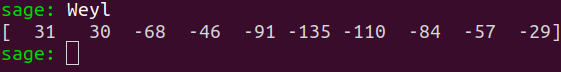
Another important character in our story is the Weyl vector (provided by Professor Shimada in his 2013 article) that can be used as Weyl vector $w_0 \in \mathbb{L}$ for an initial $\mathcal{P}_\mathbb{L}$-chamber . For instance, when $\LL = U\oplus E_{8}(-1)$, this Weyl vector $w_0$ is
Note that a Weyl vector for an initial chamber will also be automatically defined in the global namespace when $\LL$ is one of the two other lattices mentioned in the table at the beginning of this page.
You will probably have to update your initial embedding of $S$ into $\mathbb{L}$ to be able to assert that the $\mathcal{P}_S$-chamber $D_0=\DD_0 \cap \ps$ associated with this Weyl vector is contained in $\text{Nef}(X)\cap \mathcal{P}_S$ and nondegenerate, and can thus be used as starting point for the Borcherds’ for it to start exploring and processing the $\mathcal{P}_S$-chamber structure over $\text{Nef}(X)\cap \mathcal{P}_S$.
Explaining how to do so is the purpose of this page.
We, however, first have to tackle a fundamental question :
Can we apply the Borcherds’ method to the $K3$ surface under study
to obtain a generating set of its automorphism group $\aut(X)$?
We provide a criterion that will enable you to obtain an answer quickly!