NB: We provide various input data files, which can be found in the folder ThesisPrograms.
These input data files will enable you to quickly obtain a generating set of the automorphism groups
(and more) of Professor Shimada’s surfaces for many values of the parameter $k$.
Just load the input data, launch borcherds_direct, and the programs will take care of the rest.
We also provide ready-to-use input data files for almost 300 $K3$ surfaces…
The possibilities are endless; it’s up to you to take up the torch by studying other K3 surfaces…
The publication of Prof. Shimada’s 2013 article was not followed by the release of a working version of his implementation of the Borcherds’ method. However, this article contains foundational material that has been an invaluable asset for us during our PhD thesis.
As we mentioned numerous times, we owe a lot to Prof. Shimada because he laid a high-quality ground on which we were able to build during this thesis regarding the Borcherds’ method.
Despite the fact that he did not release his program, Prof. Shimada made publicly available some data regarding $K3$ surfaces he studied. We focus on Professor Shimada’s $K3$ surfaces with Néron-Severi group isomorphic to the integral lattice with Gram matrix $$\begin{bmatrix} 0 & 1 & 0 \\ 1 & -2 & 0 \\ 0 & 0 & -2k \end{bmatrix}$$ with respect to a fixed basis, where $k\in \ZZ$.
In case you read the section $9$ of Prof. Shimada’s article, you probably noticed that the case $k=11$ is used by Professor Shimada to illustrate his pioneering vision on the Borcherds’ method as an algorithmic method regarding complex algebraic $K3$ surfaces. Denote by $X$ this surface. Its Néron-Severi group $S=\NSX$ is thus isomorphic to the integral lattice with Gram matrix $$\begin{bmatrix} 0 & 1 & 0 \\ 1 & -2 & 0 \\ 0 & 0 & -22 \end{bmatrix}$$ with respect to a fixed basis.
In his 2013 article, Prof. Shimada indicates that he obtained that a generating set of the automorphism group of this surface is given by $$ \begin{bmatrix} 1 & 0 & 0 \\ 0 & 1 & 0 \\ 0 & 0 & -1 \end{bmatrix}, \qquad \begin{bmatrix} 1 & 0 & 0 \\ 11 & 1 & -1 \\ 22 & 0 & -1 \end{bmatrix}$$ and $$ \begin{bmatrix} 20 & 9 & -3 \\ 7 & 2 & -1 \\ 154 & 66 & -23 \end{bmatrix}. $$
We proceed as follows: First, we will retrieve these results using the embedding provided by Professor Shimada. Then, we will demonstrate the flexibility of our solutions and show that we can start from any primitive embedding and obtain precisely the same results.
Let’s start with Professor Shimada’s input data :
Professor Shimada provides vectors
$$ v_1 = [1,0,0,0,0,0,0,0,0,0], \quad v_2 = [0,1,0,0,0,0,0,0,0,0]$$
$$v_3 = [0, 0, 12, 8, 16, 24, 20, 16, 11, 6]$$ which define a primitive embedding $$ \iota : S \hookrightarrow \LL = U\oplus E_8(-1) $$ given by $$ \iota : [x_1 , x_2, x_3] \in S \longmapsto x_1 v_1 +x_2 v_2 + x_3 v_3 \in \mathbb{L}$$
and states that ample classes on this surface can obtained as $[3A,A,-1]$ where $A$ is a large enough integer.
We put this embedding to use and quite randomly take $A = 1024$, which should be large enough.
Note the vectors provided by Professor Shimada have coordinates given with respect to a basis for $U$ leading to a Gram matrix equal to
$$\begin{bmatrix} 0 & 1 \\ 1 & -2 \end{bmatrix}.$$
Please note that our programs were designed to be fed vectors as input (which define an embedding in an ambient lattice, check the ambient lattices table) where the basis used for $U$ yields the classical Gram matrix $$\begin{bmatrix} 0 & 1 \\ 1 & 0 \end{bmatrix}.$$ See the Toolbox section 1.3 of our thesis for more details.
You can, however, change the behavior of the programs
so that input data vectors expressed in terms of Professor Shimada’s basis for $U$ can be used, by setting
SHIMADA = Truebefore executing init_emb.
Let’s see how things work in practice. Define
v1 =  vector([1,0,0,0,0,0,0,0,0,0])
v2 = vector([0,1,0,0,0,0,0,0,0,0])
v3 = vector([0, 0, 12, 8, 16, 24, 20, 16, 11, 6])
INPUT_DATA = [ Matrix([[0,1,0],[1,-2,0],[0,0,-22]]), [v1,v2,v3],Matrix([3072,1024,-1])]
load('init_emb.sage')A warning is displayed: The sublattice of $\LL$ defined by the vectors $v_1,v_2,v_3$ does not have the desired Gram matrix.
Indeed, the program here expects you to provide vectors defined with respect to $U\oplus E_8(-1)$ using the standard basis for $U$. Still, the vectors we provided have coordinates defined with respect to the basis used by Prof. Shimada for this lattice.
We thus define
SHIMADA = Trueso that the program can consider that we work with vectors of $\LL$ having $U$-coordinates expressed with respect to Professor Shimada’s basis for $U$.
Load init_emb :
load('init_emb.sage')This time, everything is fine.
Indeed, the basis for $U$ is adapted to the coordinates of the embedding vectors provided as input data. Let’s see if we can obtain the results obtained by Prof. Shimada regarding the above-mentioned generating set of $\aut(X)$ for this surface.
NB: The Néron-Severi of the $K3$ under study contains a copy of $U$… Therefore, it is evident that things are pretty straightforward regarding two of the three embedding vectors.
Note we work on the demo server, with a default allocation of one-half of the number of logical cores available. The value of nb_workers has thus automatically been set to $4$.
Load borcherds_direct.
load('borcherds_direct.sage')The program will verify that the Borcherds’ method can be provided with a suitable initial $\ps$-chamber, will check whether an application of the method can indeed return a generating set of $\aut(X)$, and will automatically launch the method when all these requirements are fulfilled.
We readily obtain that
and see that we get results perfectly matching what was obtained by Professor Shimada a decade ago.
Let’s do things differently. Instead of using Prof. Shimada’s embedding, let’s use our own embedding vectors. Note that obtaining an initial primitive embedding should not be an issue for the study of this $K3$ surface. You can either use brute force or compute an embedding by hand. Finding primitive embedding for $K3$ surfaces of small Picard numbers should not be an issue.
This time we will work with the standard basis for $U$, and thus do not need to specify anything to the program since the latter expects to receive input data with $U$-coordinates expressed with respect to this basis.
We open a brand new sage session. The vectors
$$ v_1 = [1,0,0,0,0,0,0,0,0,0], \quad v_2 = [-1,1,0,0,0,0,0,0,0,0]$$and
$$v_3 = [0, 0, -2, 2, 2, 2, 2, 1, 1, 1]$$ define a primitive embedding $$ \iota : S \hookrightarrow \LL = U\oplus E_8(-1) $$ given by $$ \iota : [x_1 , x_2, x_3] \in S \longmapsto x_1 v_1 +x_2 v_2 + x_3 v_3 \in \mathbb{L}$$ where a Gram matrix for $U$ is $$\begin{bmatrix} 0 & 1 \\ 1 & 0 \end{bmatrix}.$$
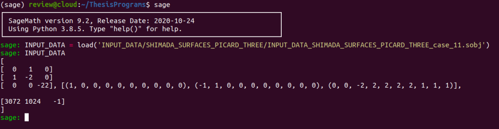
This data can be retrieved by entering
INPUT_DATA = load('INPUT_DATA/SHIMADA_SURFACES_PICARD_THREE/INPUT_DATA_SHIMADA_SURFACES_PICARD_THREE_case_11.sobj')no matter if you are on the demo server or have download our archive containing the folder ThesisPrograms and opened a Sage console from this folder.
We don’t know if this embedding will enable us to obtain an initial $\pl$-chamber $\DD_0$ having the desired non-degeneracy property. Note that we kept the same ample class as before, but keep in mind that you can use AmpTester from proj_mod to determine another ample class if you wish to do so.
Let’s try to use borcherds_direct which will perform all the checks for us :
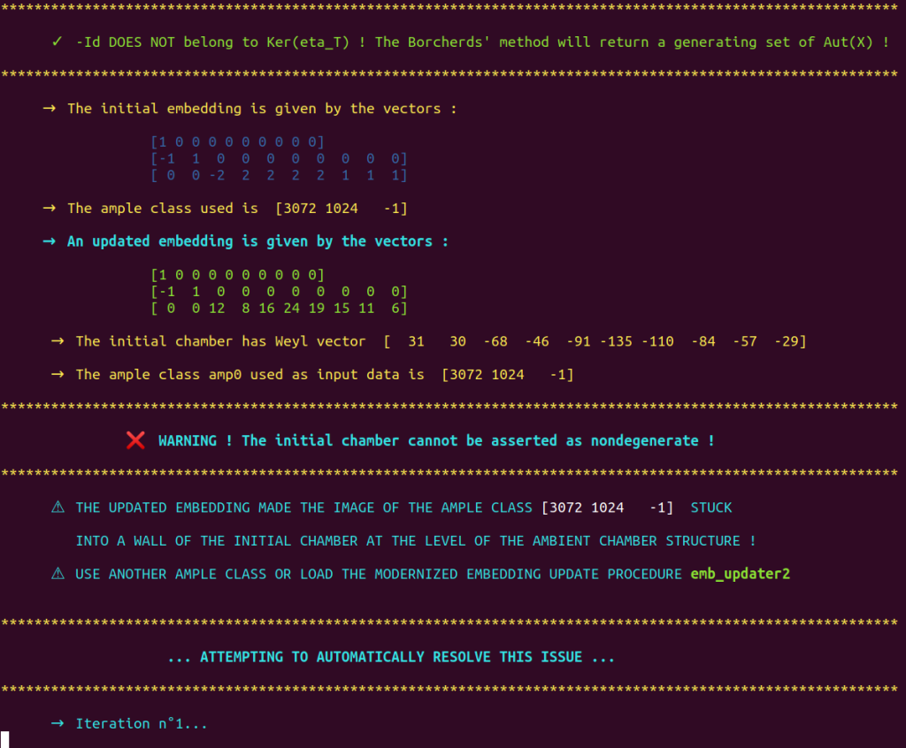
load('borcheds_direct.sage')You will see that the embedding we provided is indeed primitive. However, the program fails to assert the non-degeneracy of $\DD_0$ with the input data of our embedding and of the ample class $[3072,1024,-1]$.
Under previous versions of Borcherds’ direct, the program would have stopped: In this case, your options would have been :
- To use the program emb_updater2, which is much more efficient than emb_updater, the latter being based on Shimada’s original embedding procedure.
- To try to determine another ample class, with AmpTester from proj_mod.
The new version of borcherds_direct relies on emb_updater3. This program is an upgraded emb_updater : If everything goes fine, you will not see any difference with emb_updater.
If the latter fails to obtain a suitable embedding, emb_updater3 will use the updated embedding obtained by emb_updater as a starting point and enforce the iterative mechanics of emb_updater2, which proceeds by dynamically updating the embedding, see the section 1.8.3 of our thesis for more details. By default, the program will try to resolve the issue with the updated embedding by applying at most $5$ iterations of emb_updater2.
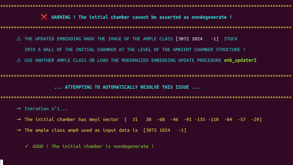
The maximum number of iterations of emb_updater2 performed by emb_updater3 can be controlled by assigning the value of your choice to the variable max_iter. Otherwise, the value of this variable will be set to $5$.
Regarding the surface under study and the embedding we provided, one iteration is enough to obtain an embedding that enables borcherds_direct to assert the nondegeneracy of $\DD_0$ :
The Borcherds’ method is then automatically executed and outputs exactly the results which have been obtained earlier when we used Shimada’s embedding :
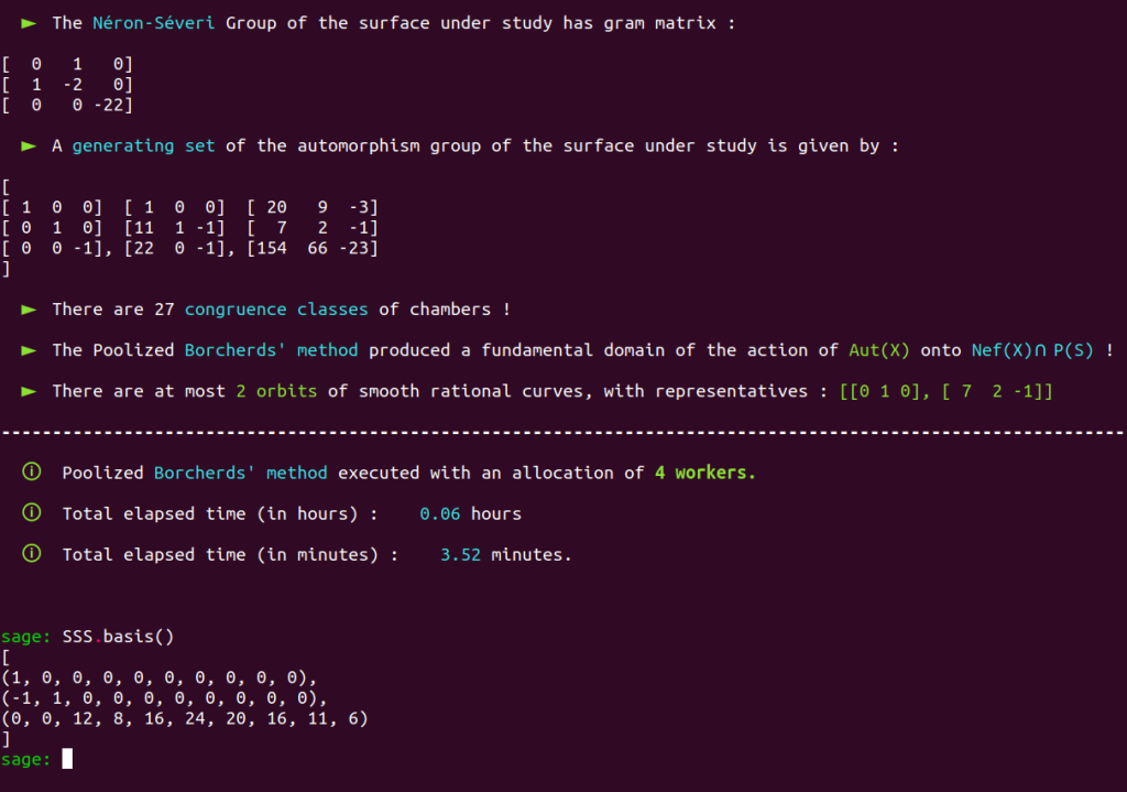
If you look at the above picture, you will notice that we obtained Professor Shimada’s embedding thanks to the embedding update procedure and did not even have to break a sweat to do so. Note that the first two vectors, which have non-zero $U$-coordinates, are expressed with respect to the standard basis for $U$, while Shimada’s vectors have $U$-coordinates expressed with respect to his basis for this lattice.
As displayed above, the Borcherds’ method produced a fundamental domain of the action of $\aut(X)$ onto $\nps$. We launch fundamentalizer in order to study this fundamental domain
and obtain that an Hilbert basis of the convex cone associated to the fundamental domain of the action of $\aut(X)$ onto $\nps$ is $$\left[2, 1, 0\right], \left[1, 0, 0\right], \left[14, 7, -2\right], \left[21, 8, -3\right], \left[8, 2, -1\right], \left[8, 4, -1\right], \left[7, 3, -1\right] $$ with intersection matrix $$\begin{bmatrix} 2 & 1 & 14 & 21 & 8 & 8 & 7 \\ 1 & 0 & 7 & 8 & 2 & 4 & 3 \\ 14 & 7 & 10 & 15 & 12 & 12 & 5 \\ 21 & 8 & 15 & 10 & 8 & 18 & 5 \\ 8 & 2 & 12 & 8 & 2 & 10 & 4 \\ 8 & 4 & 12 & 18 & 10 & 10 & 6 \\ 7 & 3 & 5 & 5 & 4 & 6 & 2 \end{bmatrix}$$