Study of automorphism groups,
orbits of smooth rational curves
In order to fulfill our goals regarding the first two points appearing in the title of this thesis, that is, the study of automorphism groups and the study of orbits of smooth rational curves, we built on Shimada’s 2013 work and provided an accessible, fully functional and generalized implementation of the Borcherds’ method which also takes advantage of process-based parallelism, and more generally, of parallelism at a broader scale.
Let us show how things work by studying a surface belonging to the family of surfaces $X_t$ with Picard number $3$. Studying these surfaces (automorphism groups and orbits of $(-2)$-curves) was the goal to be achieved in order to complete our PhD thesis.
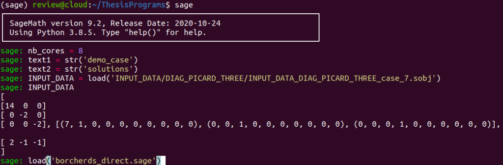
For instance, assume that the surface under study is the $K3$ surface $X_7$ with Néron-Severi group $S_7 = \text{NS}(X_7)$ isomorphic to the integral lattice with the following Gram matrix with respect to a fixed basis :
We show in the section 2.3 of our thesis that the class $[2,-1,-1]$ can be taken as an initial ample class on a surface such as $X_7$.
The elements $$v_1 = [7,1,0,0,0,0,0,0,0,0], \; \, v_2 = [0,0,1,0,0,0,0,0,0,0] \; \ \text{and} \,\; v_3 = [0,0,0,1,0,0,0,0,0,0]$$
define a primitive embedding of $S_7$ into $\mathbb{L}=U\oplus E_8(-1)$.
This is all the input data we need in order to launch the Poolized Borcherds’ method.
From now on, we assume that the reader either uses the demo server or opened a Sage console from our folder ThesisPrograms contained in our programs bundle, so that everything we do, you can do too without hassle simply by copying and pasting commands.
We just have to specify the minimal input data we just discussed, and let borcherds_direct work for us. If the Borcherds’ method cannot be applied to the surface under study (e.g. kernel condition not satisfied, embedding not primitive, initial embedding which cannot be updated automatically to obtain a suitable initial chamber….), the program will obviously not launch the method.
We will often voluntarily put us in unfavorable positions in order to show you the flexibility and scope of application of our tools. Demonstrating our solutions in 100% controlled situation on pre-studied cases for which we already know in advance that everything will be fine would not only be unfair to our readers, but would also be a waste of time for all of us.
The program borcherds_direct is simply a series of nested Boolean checks each testing one of the major conditions which have to be satisfied by the surface under study in order to execute the Borcherds’ method and obtain a generating set of $\text{Aut}(X)$ :
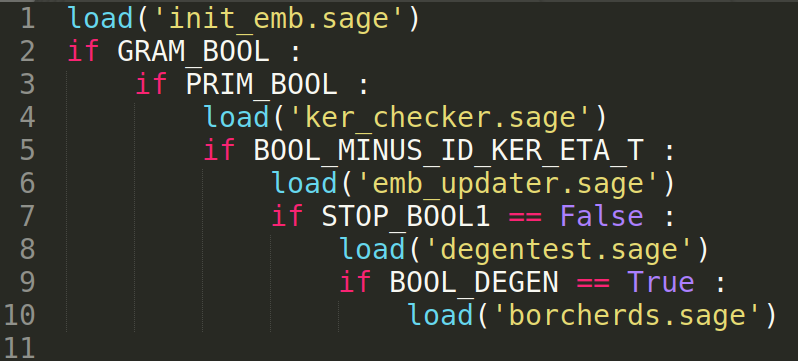
We launch the program :
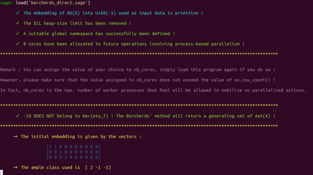
The program suddenly stops :
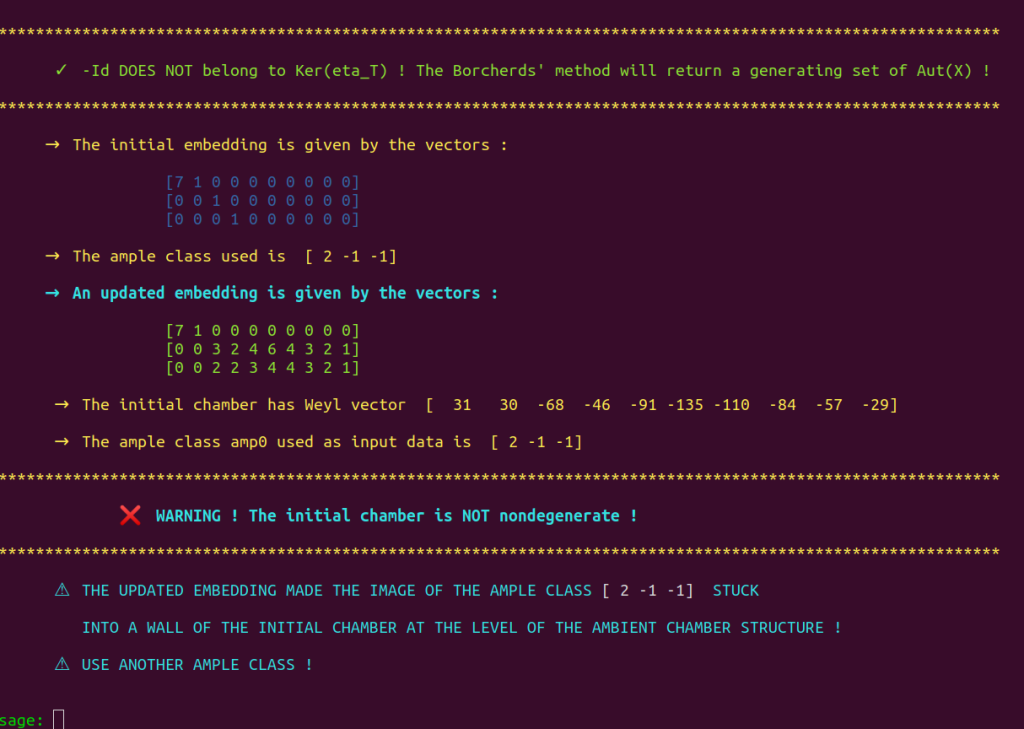
We are here facing one of the limit cases of Shimada’s embedding update procedure : The image $\iota_\text{upd}(a_0)$ of the ample class $a_0 = [2,-1,-1]$ under the updated embedding $ \iota_\text{upd} : S \hookrightarrow \mathbb{L} $ is stuck into a wall a the initial $\mathcal{P}_{\mathbb{L}}$-chamber $\mathcal{D}_0$. See section 1.8 of our thesis for more details.
We therefore use another ample class, which will hopefully work.
In order to do so, we use our program AmpTester, which enables us to determine whether any class in the Néron-Severi group is ample or not, as long as we have knowledge of a Gram matrix of the Néron-Severi and of the data of an initial ample class. This is here the case.
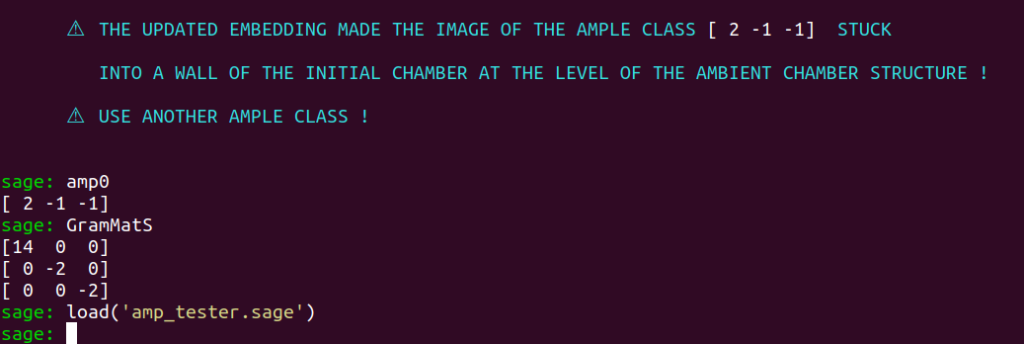
First, we make sure that the initial ample class can be found under the variable name amp0 and that the Gram matrix is assigned the variable GramMatS.
We then load amp_tester :
If you don’t know what to do, you can then try as many classes as you desire until AmpTester indicates that the class used as input data is ample.
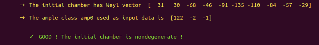
In our case, we will give a try to the class $[122,-2,-1]$ :
AmpTester(Matrix([122,-2,-1]))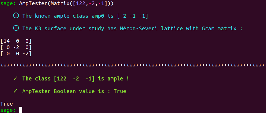
Great ! Let’s give a try again with this new ample class. First, we have to update the input data list, as follows :
INPUT_DATA[2] = Matrix([122,-2,-1])
INPUT_DATA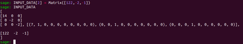
We can launch borcherds_direct again :
This time, things went fine :
and the program immediately launches the Borcherds’ method :
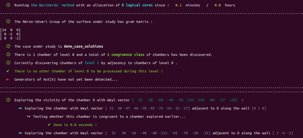
which returns a generating set of $\text{Aut}(X)$ and a list of representatives of all the orbits of smooth rational curves on $X$.
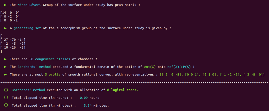
An AMD 5950X can perform the same computation in only 2 minutes, with an allocation of 16 logical cores out of 32 (which is anyways quite useless on such a basic case with so few chambers).
Note that the Borcherds’ method also provided a fundamental domain of the action of $\text{Aut}(X)$ onto $\nps$. Let’s study this fundamental domain with our program fundamentalizer :
This program starts by precisely determining the geometry of the fundamental domain by identifying its boundary walls (see section 1.9 of our thesis for more details) :
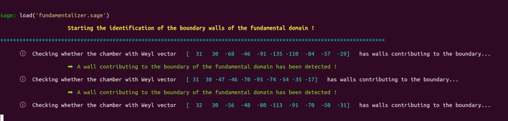
fundamentalizer then displays the list of boundary walls of the fundamental domain :
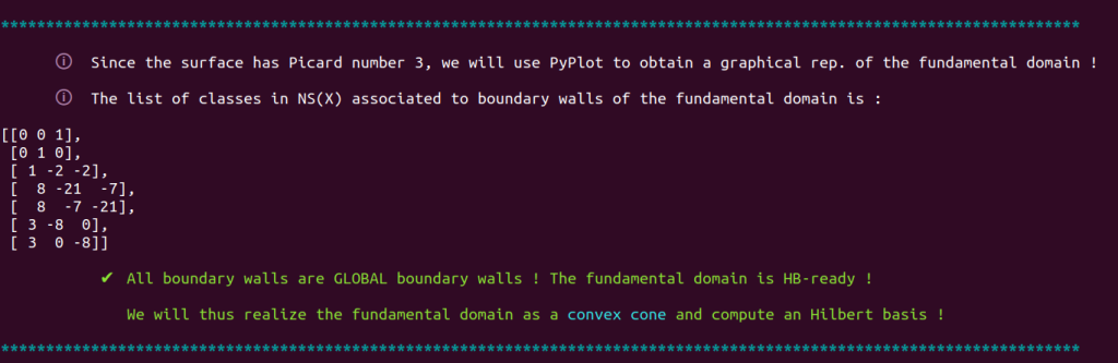
and indicates in this case that the fundamental is HB-ready (see section 1.9.2 of our thesis) and can thus be realized as a convex cone to compute an Hilbert basis.
This Hilbert basis will be quite interesting, since the fundamental domain is a chunk of the the Nef cone !
fundamentalizer then displays the Hilbert basis of this cone :
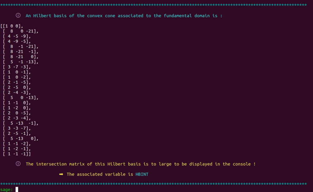
and indicates that the matrix is too big to be displayed properly in the console.
Let’s take a look a a chunk of this matrix, for example its $15 \times 15$ upper left diagonal submatrix :
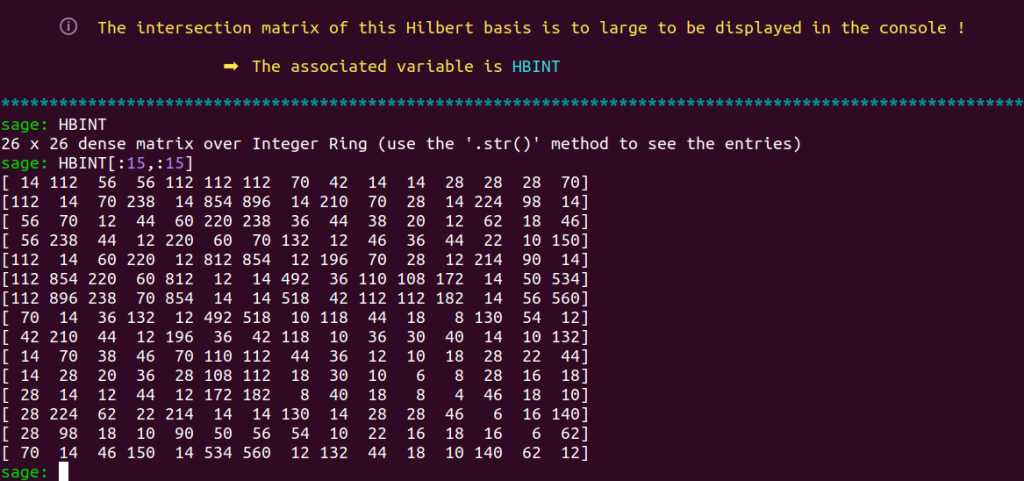
It looks quite nice, isn’t it ?
We now use fundamentalizer to obtain a graphical representation of the fundamental domain. To this end, we set PLOT_BOOL = True and launch fundamentalizer again.
The program will prompt us to type
plt.show()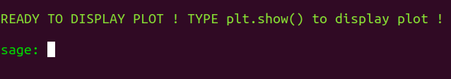
And a graphical representation of the fundamental domain as an object on the $\mathcal{P}_S$-chamber structure will appear
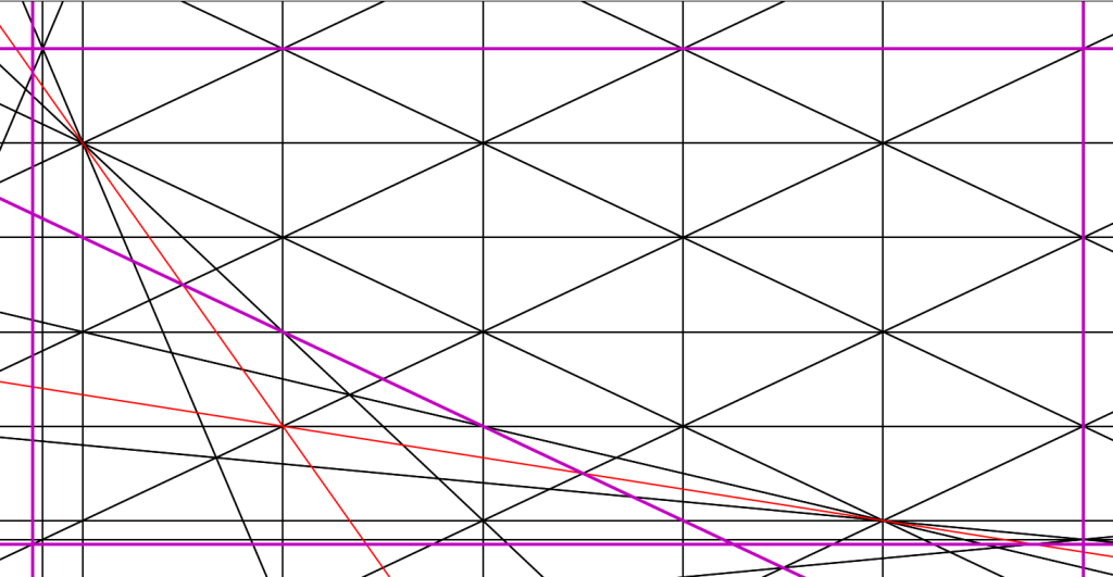
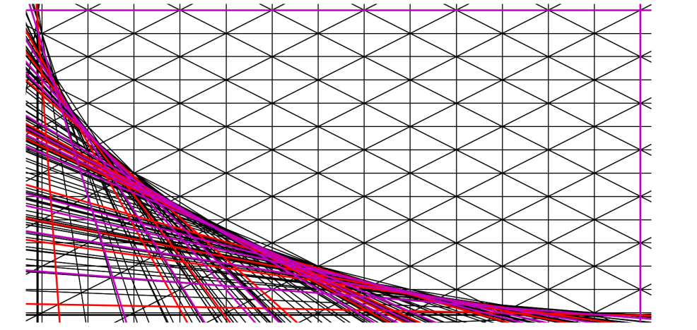
With a bit of post-processing, this fundamental domain becomes
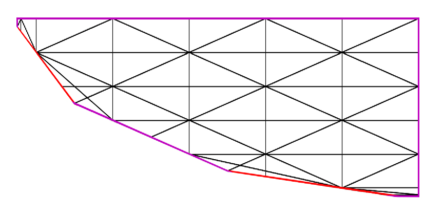
These figures are interesting : Note that if you tweak the program in order to display classes of smooth rational curves you computed with Xavier Roulleau’s SmoothRationalCurves ( available in Sage / Python through CGS ), you will see that the the curves accumulate in such a way which perfectly fits the shape the basic figure produced by fundamentalizer.
I do not have the picture in hand for $X_7$, but I can show you how it looks like for $X_{43}$, for example :