A classical case, which can be found in Billard’s 2003 article and originates from Joachim Wehler’s 1988 article K3-surfaces with Picard number 2, is the $K3$ surface $X$ with Néron-Severi group $S=\NS(X)$ isomorphic to the integral lattice with Gram matrix $$G_S =\begin{bmatrix}0 & 2 & 2 \\ 2 & 0 & 2 \\ 2 & 2 & 0 \end{bmatrix}$$ with respect to a fixed basis.
This $K3$ is known to have an automorphism group generated by
$$ \begin{bmatrix}1 & 2 & 0 \\ 0 & -1 & 0 \\ 0 & 2 & 1 \end{bmatrix},\begin{bmatrix} 1 & 0 & 2 \\ 0 & 1 & 2 \\ 0 & 0 & -1 \end{bmatrix}, \begin{bmatrix} -1 & 0 & 0 \\ 2 & 1 & 0 \\ 2 & 0 & 1\end{bmatrix}$$as indicated in Billard’s 2003 article.
Note that the convention used by Billard is that matrices $ M \in O(S)$ satisfy $$ M^t G_S M = G_S. $$Since we used throughout our thesis the convention that matrices $M\in O(S)$ instead satisfy $ M G_S M^t = G_S $, we will take the transpose of each of these matrices and write them so as to satisfy the convention which suits the tools we use :
$$\begin{bmatrix} 1 & 0 & 0 \\ 2 & -1 & 2 \\ 0 & 0 & 1 \end{bmatrix}, \begin{bmatrix} 1 & 0 & 0 \\ 0 & 1 & 0 \\ 2 & 2 & -1 \end{bmatrix}, \begin{bmatrix} -1 & 2 & 2 \\ 0 & 1 & 0 \\ 0 & 0 & 1 \end{bmatrix}$$
Can we use the Borcherds’ method to obtain these results ? Let’s try !
The elements $$v_1 = [1, 1, -1,0,0,0,0,0,0,0], \; \, v_2 = [2, 2, 0, 2, 2, 2, 2, 1, 0, 1] \; \ \text{and} \,\; v_3 = [1, 1, 0, 1, 0, 0, 0, 0, 0, 0]$$
define a primitive embedding of $X$ into $\mathbb{L}=U\oplus E_8(-1)$.
One can easily show that the class $[1,1,1]$ can be taken as an initial ample class on this surface (there are no $(-2)$-curves on this surface; thus, ampleness is not an issue on this surface).
If you are currently logged on the demo server, proceed as follows :
INPUT_DATA=load('INPUT_DATA/DEMO/INPUT_DATA_WEHLER_PICARD_THREE.sobj') We define
text1 = str('wehler_1988')
text2 = str('demo')
and directly launch the program borcherds_direct, which will automatically stop if one of the conditions that must be fulfilled to execute the Borcherds’ method is not met.
load('borcherds_direct.sage')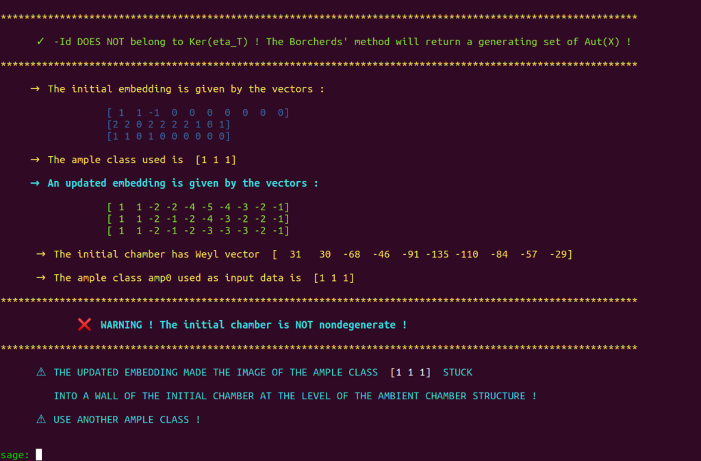
We quickly see that there is an issue with the ample class, whose image under the updated embedding is stuck straight into a wall of the initial $\mathcal{P}_{\mathbb{L}}$-chamber $\mathcal{D}_0$.
Be careful because Shimada’s 2013 approach would lead you to use a trial and error-based method to escape this dire situation.
A decade later, we provide a universal ampleness tester (and modernized embedding update procedures). Let’s make use of AmpTester and find another ample class.
NB: There are no $(-2)$-curves on these surfaces, so testing for ampleness is not a necessity,
but we do so for the sake of illustrating how to use AmpTester
Load proj_mod and enter
AmpTester(Matrix([1000,100,10]))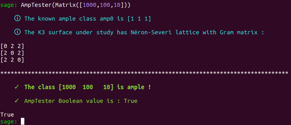
Fine, let’s use $[1000,100,10]$ as our new ample class :
amp0 = Matrix([1000,100,10])AGAIN, please note that using AmpTester is not needed here!
Since there are no $(-2)$-curves on this surface, we can take any class with
a strictly positive square as an “ample” class… We, however, use AmpTester for the sake of showing our tools in action.
We then launch emb_updater followed by degentest :
load('emb_updater.sage')
load('degentest.sage')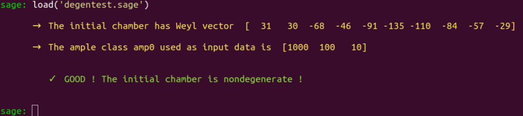
Good! We can launch the Borcherds’ method!
load('borcherds.sage')
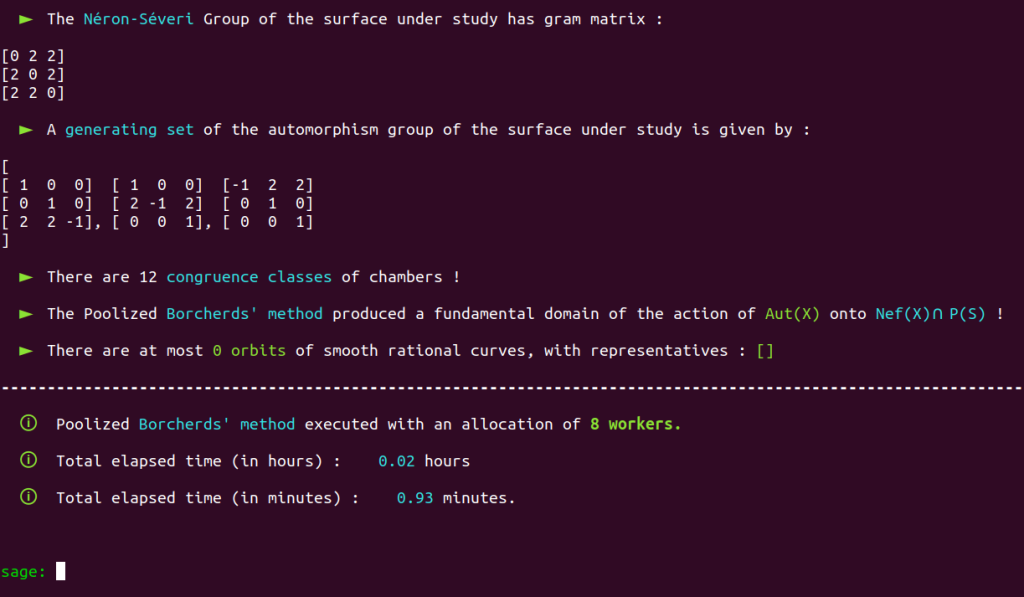
We thus see that the Borcherds method precisely returns the generating which can be found in classical references (such as Billard) $$\begin{bmatrix} 1 & 0 & 0 \\ 2 & -1 & 2 \\ 0 & 0 & 1 \end{bmatrix}, \begin{bmatrix} 1 & 0 & 0 \\ 0 & 1 & 0 \\ 2 & 2 & -1 \end{bmatrix}, \begin{bmatrix} -1 & 2 & 2 \\ 0 & 1 & 0 \\ 0 & 0 & 1 \end{bmatrix}$$ and we note that doing so by enforcing our computed-based approach takes no more than 60 seconds on our demo server, which is quite “average” in terms of raw processing power. Note that there are no orbits of smooth rational curves, since there are not such curves on this surface.
Since there are no $(-2)$-curves on these surfaces, and thus no curve of strictly negative self-intersection on this $K3$ surface, we, therefore, deduce that $$\nef= S$$ where $S=\NSX$ and hence $\nps$ coincides with $\ps$.
The fundamental domain of the action of $\aut(X)$ onto $\nps$ it thus a fundamental of $\ps$ under the action of $\aut(X)$. The associated cone, which includes the boundary (made of classes of square $0$) should have a Hilbert basis that spans $\NSX$.
We use fundamentalizer to study the fundamental of $\ps$, under the action of $\aut(X)$ returned by the Borcherds’ method and check whether such an Hilbert basis can be obtained :
load('fundamentalizer.sage')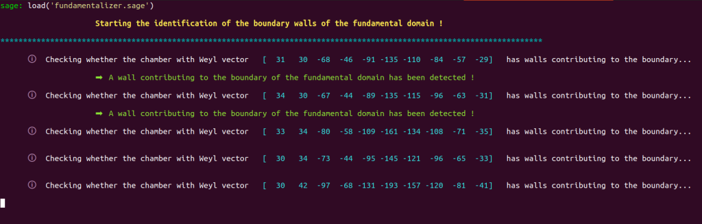
We obtain :
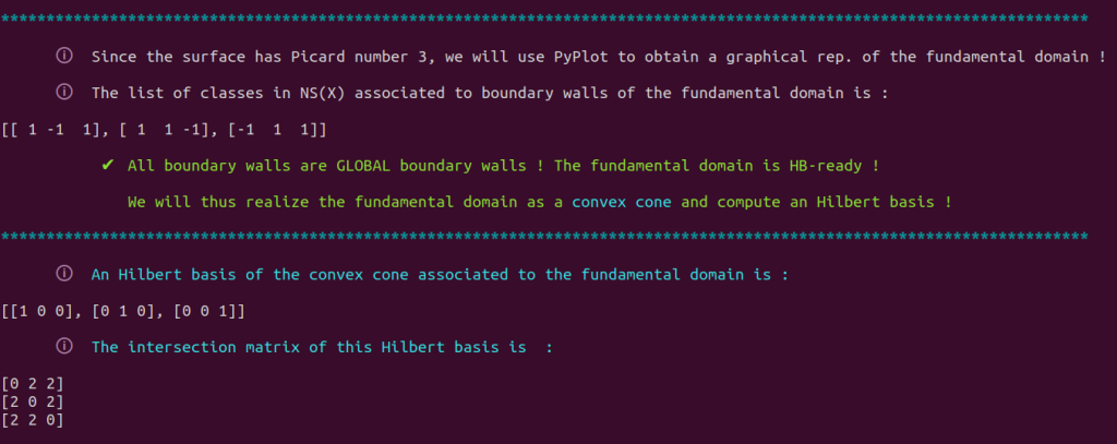
An Hilbert basis of the convex cone associated to the fundamental domain is therefore
$$ [1,0,0], [0,1,0], [0,0,1]$$
and an intersection matrix of this basis is
$$\begin{bmatrix}0 & 2 & 2 \\ 2 & 0 & 2 \\ 2 & 2 & 0 \end{bmatrix}.$$
As expected, this Hilbert basis spans $\NSX$.
We now use fundamentalizer to obtain a graphical representation of this fundamental domain.
PLOT_BOOL = True
load('fundamentalizer.sage')
Type
plt.show()NB: will not display anything on the demo server’s console… You have to run this example on your computer to use PyPlot graph rendering. You can directly pull the folder ThesisPrograms from the demo server or download ThesisPrograms.zip)
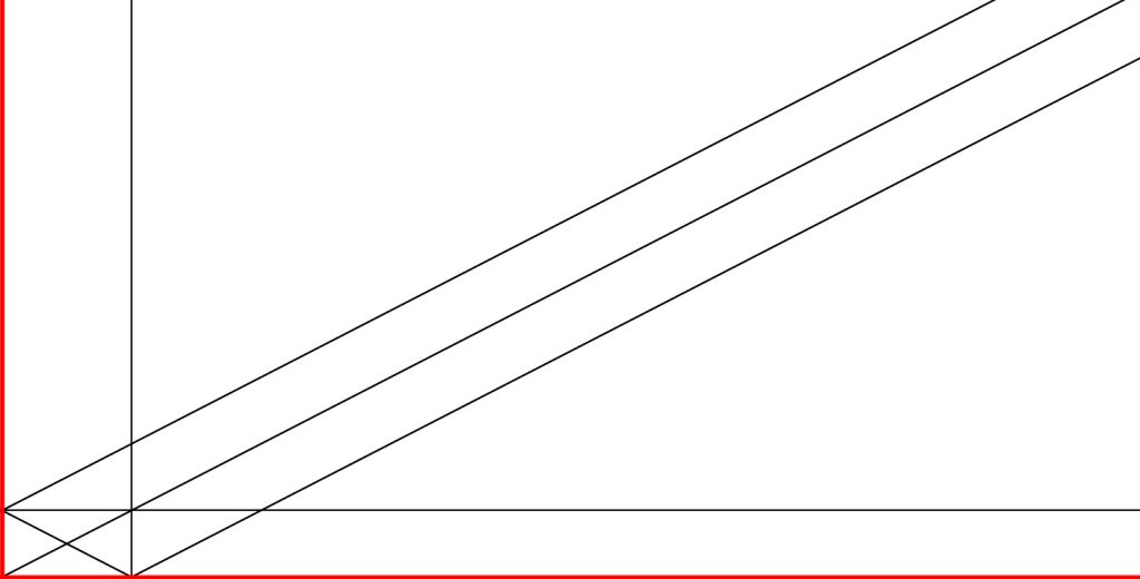
We can observe that there are twelve chambers and that this domain is not closed. This situation can be explained by the absence of smooth rational curves on the surface under study.